Linear Safety Probes Cannot Silence Features They Detect
TL;DR. A linear probe direction is asked to do three jobs: detect the feature, steer by adding it, and silence by projecting it out. Only silencing is the necessity test. On four open-weights families (Llama-3-8B, Gemma-2-9B, Mistral-7B-v0.3, OLMo-2-7B) and two features (refusal, sycophancy), I find probes that detect at AUROC ≥ 0.91 and steer cleanly yet fail to silence. The failure is recipe-specific: difference-of-means (DoM) and cross-validated logistic regression (LR-CV) have disjoint failure sets, so no fixed recipe is safe. A single cosine at calibration time predicts which recipe silences, and a calibration check built on it recovers 17/17 causal handles on a 22-cell battery and alarms on the remaining 5.
Epistemic status. Four families, two features, 35 whitening cells, a 22-cell cross-family battery plus a 5-cell held-out Qwen2.5-7B replication. Numbers hold; the generalization to novel architectures, feature types, and non-linear monitors is the open question. Full paper here.
The gap, restated
Imagine you’re standing up a safety case on top of a linear probe. It classifies activations as “about to refuse” vs “about to comply.” It passes the standard checks: AUROC 0.94 on held-out data; additive steering along the probe direction monotonically reduces refusal with a clean dose-response. You ship.
What you haven’t tested is whether the direction your monitor watches is the axis the model uses to produce the behavior. That’s a separate property, and it’s the one the deployment actually needs. The test is Arditi-style projective ablation: project the probe direction out of the residual stream at every token. If behavior drops, the direction is the causal axis. If it doesn’t, the direction was reading a correlated proxy — the probe detects, you can push against it, but the model routes around it whenever you aren’t pushing.
Anthropic’s Claude Mythos Preview system card flagged this qualitatively:
“The causal effects of individual features often changed over the course of post-training, making it difficult to attribute behavioral changes merely to increases or decreases in particular feature activations.” — Mythos Preview System Card, §4.5.3.4
My first paper measured one instance of this gap: frozen probes pass detection and steering tests but fail necessity after fine-tuning. This paper shows the gap is there before any further training — at calibration time, on the freshest possible probe fit to the current checkpoint. It’s not a fine-tuning artifact. It’s a fact about the geometry of labeled buffers.
Three jobs, one direction
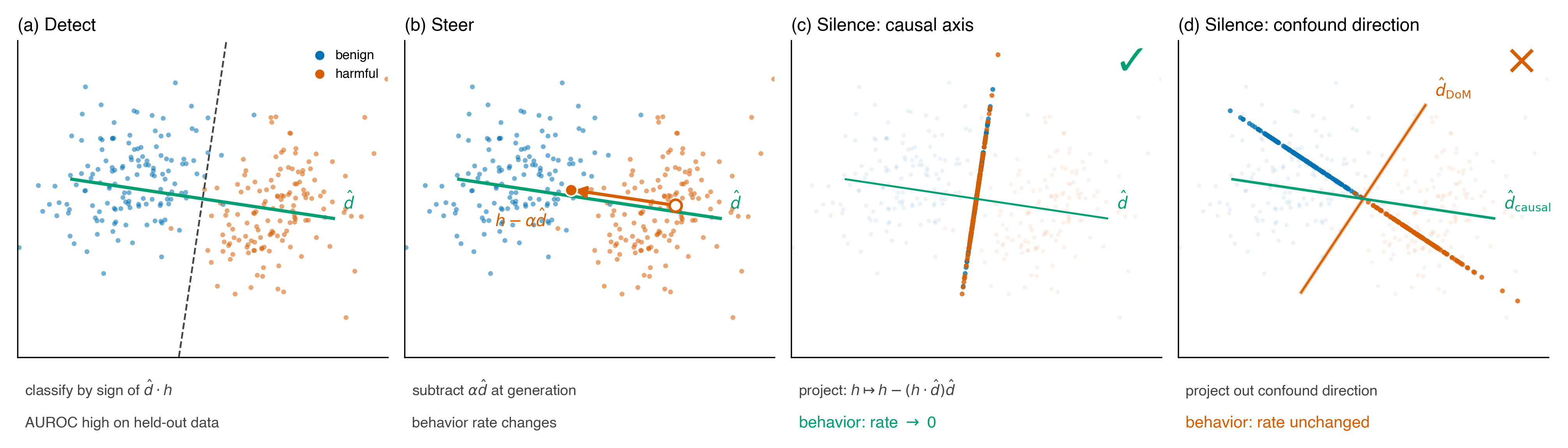
The three-jobs picture is the whole frame. Detect and steer pass on both (c) the causal axis and (d) a within-class confound. Only silencing reports the difference. A safety case built on “the probe detects and we can steer” is implicitly assuming detect–steer–silence collapse to one direction. Under identical-covariance Gaussian classes they do. In practice, they often don’t.
The hero result: the recipe that works depends on the model
I ran the three tests on two extraction recipes (DoM and LR-CV) at the per-family peak probe layer, across four open-weights families, each with four rounds of benign UltraChat SFT. Every (model, feature, recipe) panel hits AUROC ≥ 0.91 on held-out data. Every panel produces monotone dose-response under additive steering.
The silencing verdicts diverge.
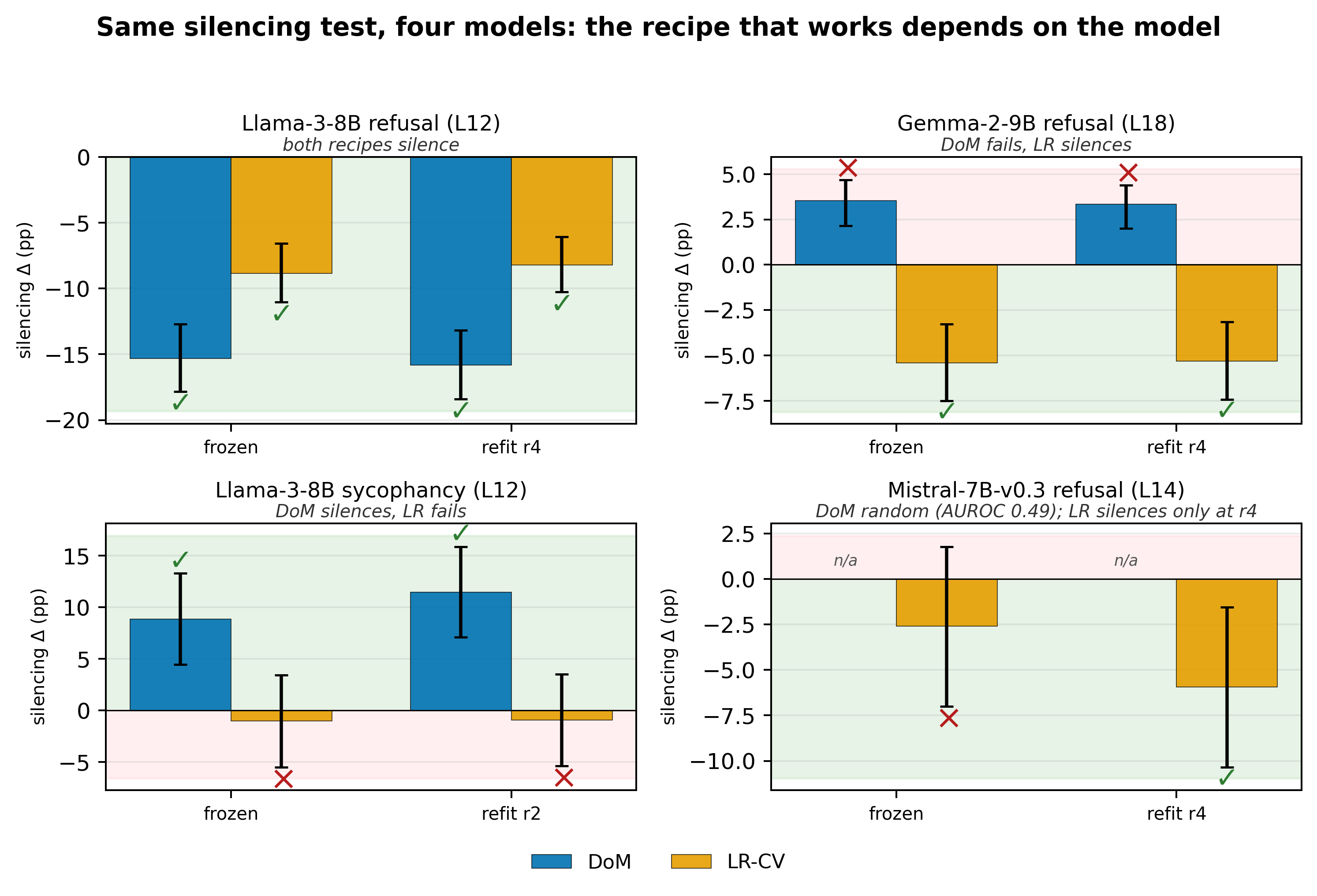
- Llama-3 refusal (L12): both recipes silence. Either direction is the causal axis.
- Gemma-2 refusal (L18): DoM fails with the wrong sign (+3pp — projecting it out raises refusal). LR-CV silences cleanly. Picking DoM here silently inverts your intervention.
- Llama-3 sycophancy (L12): roles flip. DoM silences (+10pp, anti-sycophancy direction). LR-CV does nothing.
- Mistral-7B-v0.3 refusal (L14): DoM AUROC 0.49 — random. LR-CV detects at AUROC ≥ 0.91 at every checkpoint but only silences at the most-trained one. At the first three checkpoints, no linear direction at any body layer silences refusal, yet LR-CV detects it cleanly throughout.
The two recipes’ failure sets are disjoint. There is no fixed choice of recipe that silences across the battery. Mistral is the cleanest existence proof: detection and steering are fine; silencing reports that the feature is not linearly accessible at all. A monitor watching detection and steering reads healthy while the intervention does nothing.
The mechanism: a within-class confound
The class mean μ⁺ − μ⁻ is Bayes-optimal when the two classes have identical covariance. That assumption fails when within-class variance carries a label-correlated surface feature v — something like formality or sentence length that shifts systematically between the feature-positive and feature-negative buffers at the probe layer. In that regime:
d̂DoM = α · (causal axis) + β · (confound)
When β dominates, projecting plain DoM out removes v and little of the axis you wanted to silence. LR-CV is less susceptible because held-out regularization penalizes directions that generalize poorly across folds — typically surface confounds. That’s the asymmetry.
The decomposition is testable. Project out the top within-class principal components first, refit DoM on the whitened activations, and three regimes should appear: recovery when β dominates, preservation when α dominates, near-noop as β → 0. They do:
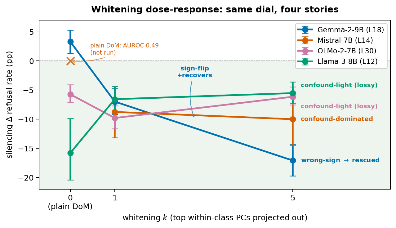
- Gemma-2 (wrong-sign → rescued): Δ flips from +3pp at k=0 to −17pp at k=5. The top PCs carried the confound; peeling them off exposes the causal axis.
- Mistral (confound-dominated → rescued): plain DoM random at every layer; whitening at k=1 recovers silencing at every cell (−10 to −5pp).
- Llama-3 / OLMo-2 (confound-light): plain DoM is already the causal axis; whitening is mildly lossy.
- Llama-3 sycophancy (confound-free): cos(plain, whitened) = 1.00; whitening is a noop.
Same dial, four stories. The dial is within-class confound mass.
One cosine predicts silencing
If the decomposition is right, one calibration-time scalar should be enough to tell the regimes apart: the cosine between plain DoM and DoM refit on whitened activations.
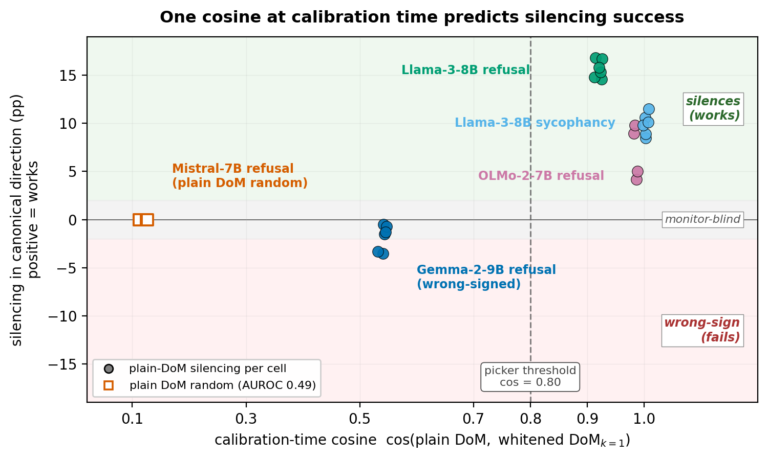
The cosine tracks silencing monotonically across 35 cells spanning [0.12, 1.00]:
- cos ≈ 0.1 (Mistral) → plain DoM is random. Confound-dominated.
- cos ≈ 0.5 (Gemma-2) → plain DoM is wrong-signed. Projecting it out raises the behavior.
- cos ≥ 0.8 (Llama-3, OLMo-2, Llama-3 sycophancy) → plain DoM silences.
The 0.80 threshold sits in the empirical gap [0.55, 0.92] between the confound-dominated and confound-light clusters. Any threshold in that range routes every body-battery cell identically.
The calibration check
The cosine observation converts into a one-line deployment protocol. At every checkpoint, on a labeled buffer of feature-positive and feature-negative activations at the per-family probe layer:
- Fit plain DoM. Fit whitened DoM (top within-class PC projected out). Compute cos.
- If cos ≥ 0.80, the picker selects plain DoM. Else whitened DoM.
- Project the picked direction out at every token. Report a 95% Newcombe CI on the behavior-rate change.
- If the CI excludes zero in the task-canonical sign, adopt the direction as the causal handle. Otherwise the alarm fires: no linear direction at this layer silences this feature at this checkpoint.
On the 22-cell four-family battery, the picker recovers all 17 causal handles that exist and correctly alarms on the remaining 5. Fixed-DoM alone recovers 10/22. Fixed-LR-CV alone recovers 13/22. A held-out Qwen2.5-7B replication with the threshold frozen before that family ran adds 5 confound-light cells; the picker routes all five to DoM without retuning. Marginal cost: one extra probe fit and one extra projection per checkpoint.
What this changes for probe-based safety monitors
Three concrete changes for anyone shipping a linear probe as a runtime monitor:
- Sweep layers per family. OLMo-2’s causal axis is at L30 on a 32-layer model. An L12–L18 convention would miss it entirely. The peak detection layer is not a constant across architectures.
- Compute cos(plain DoM, whitened DoM) at calibration. It’s one scalar and it tells you whether plain DoM is the causal axis or a confound before you run any silencing experiments. A low cosine is a red flag, not a tuning detail.
- Report a 95% CI on the silencing Δ. Treat a CI that includes zero as an alarm, not a tuning signal. Detection and steering passing is not a substitute — that’s the whole point of the Mistral result.
Where this sits in the bigger picture
The first paper showed probes can pass detection tests and fail necessity after fine-tuning. This one shows they can fail necessity from the start, on the freshest possible probe fit to the current checkpoint. The sufficiency–necessity gap is not a fine-tuning artifact; it’s a calibration-time fact about the geometry of labeled buffers. Both failures are silent — the monitor reads healthy while the intervention does nothing — and both are avoidable with a necessity check that costs one extra projection.
The deeper claim is the same across both papers: probe accuracy is not evidence of a causal handle. Deploying model-internals probes as safety interventions requires a necessity test, not just a detection score.
Open questions
- Name the confound. On Mistral at L14 the top within-class PC carries enough mass that plain DoM is a random direction. Best guess: the AdvBench-vs-Alpaca register gap (imperative and stripped-down vs. conversational), but it’s untested. Extracting the PC, steering with it, and identifying what linguistic property it encodes would convert the α·(causal) + β·(confound) account from a structural decomposition into a mechanistic one.
- Beyond refusal. The decomposition is feature-agnostic. Whether it extends to deception-detection probes, capability-elicitation probes, or SAE-feature stability under fine-tuning is what distinguishes a refusal-specific geometric fact from a general failure mode of linear probe-based monitors.
- Multi-layer. Single-layer silencing Δ of 5–17pp is too large for standard backup-head routing to explain cleanly, but the multi-layer replication across the full battery is outstanding.
Limitations
Refusal on four families + sycophancy on Llama-3. 35 whitening cells in total. Enough to establish the cosine-signature monotone across [0.12, 1.00]; not enough to predict which regime a novel family falls into from pretraining metadata alone. Projective ablation is a necessity test subject to a self-repair caveat — the operational claim is about the deployed layer. The setup is linear only; I characterize the calibration-time dissociation, not arbitrary training dynamics.
If you run deployment monitors on production models, I’d like to know whether your protocol would alarm on a probe that detects cleanly but produces no silencing effect. Comments welcome.